

Laser beam propagation is essential for understanding how a laser interacts with optical systems. One of the key methods for modeling laser beam propagation is the ray-based approach, which is widely used in optics for its simplicity and efficiency. Below is an overview of the process and how it can be applied in modeling a laser beam using this method.
Introduction to Laser Beam Propagation
OpticStudio sequential mode offers three primary tools to model Gaussian beam propagation:
- Ray-based Approach: This method uses geometrical ray tracing to simulate beam propagation.
- Paraxial Gaussian Beam Analysis: A method for modeling Gaussian beams and obtaining detailed beam parameters.
- Physical Optics Propagation (POP): This method models the beam by propagating a coherent wavefront, providing detailed insights into arbitrary coherent optical beams.
This article focuses on the ray-based approach.
Gaussian Beam Theory
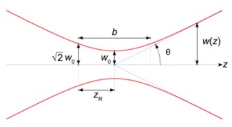
A Gaussian beam is an idealized beam with a specific waist (w0). The properties of the beam can be described using three key parameters:
- Wavelength (λ): The wavelength of light.
- Beam Waist (w0): The beam’s minimum radius at the waist.
- Divergence Angle (θ): The angle at which the beam spreads as it propagates.
As illustrated in the schematic diagram, the Gaussian beam size is a function of its distance from the waist. The equation for the beam width (w(z)) is:
w(z) = w0 [ 1 + (z/zR)^2 ]^(1/2)
Where:
- z is the distance from the waist.
- zR is the Rayleigh range of the beam.
For large distances, the beam expands linearly, and the divergence angle (θ) is given by:
θ = λ / (π * w0) for z >> zR
Where:
- zR is the Rayleigh range, calculated by:
zR = π * w0² / λ
This shows how the beam size increases with distance and helps us calculate the focal spot or beam divergence.
Ray-Based Approach to Model Gaussian Beam Propagation
The ray-based approach uses geometrical optics to model the propagation of a Gaussian beam. Rays are imaginary lines that represent the path of light, typically perpendicular to the wavefronts.
In the ray-based model:
- Inside the Rayleigh range (z < zR), the beam propagates slowly, and the size changes minimally. Here, we can model the beam as a collimated ray bundle.
- Outside the Rayleigh range (z >> zR), the beam diverges, and we can model it as a point source for simplicity.
This is useful in systems where beam size changes slowly over short distances but diverges significantly over larger distances.
Example Setup
Consider a laser beam with a wavelength of 355 nm and measured divergence of 9 mrad at a surface 5 mm from the laser output. Using this information, we calculate the waist location, beam size, and divergence using the ray-based approach.
- Nominal Wavelength: 355 nm
- Measured Divergence: 9 mrad
- Beam Diameter: 2 mm
The beam waist location is calculated using the beam divergence and Rayleigh range. By inputting the measured divergence into the Merit Function Editor in OpticStudio, we can optimize the beam focusing system.
Optimizing the Beam Focusing System
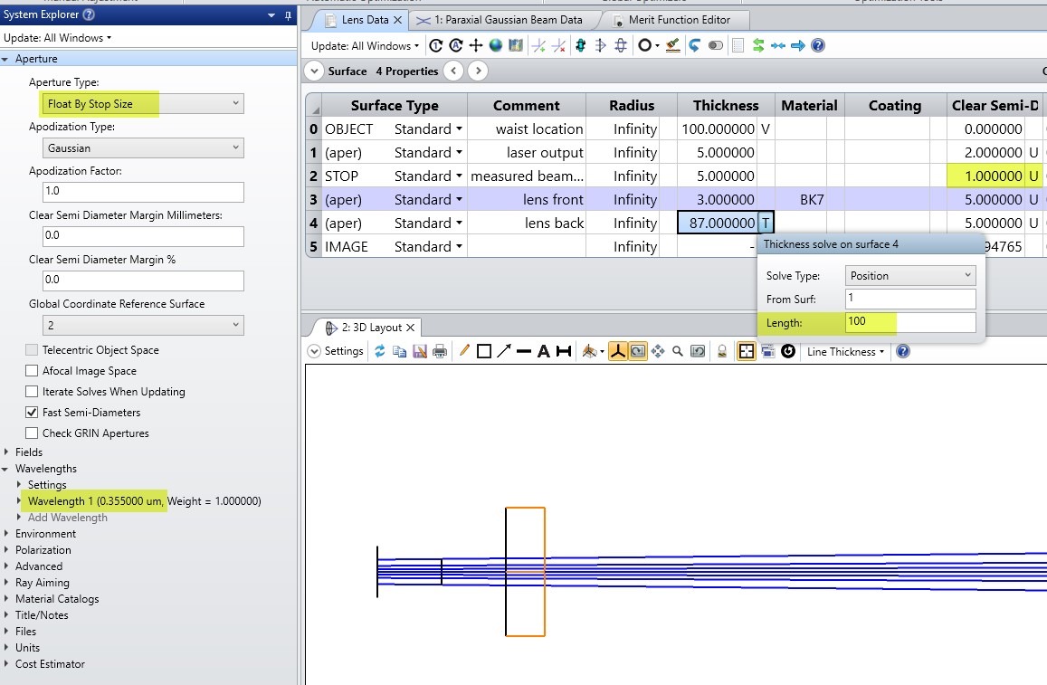
To optimize the system, we calculate the minimum spot size at 100 mm from the laser output. The process involves adjusting the lens positioning to achieve the smallest possible focus.
Steps for Optimization:
- Set the input beam parameters in the OpticStudio system explorer.
- Use the ray-based approach to calculate beam divergence and waist location.
- Optimize the lens using the Optimization Wizard to focus the beam with minimal spot size.
This process helps achieve the smallest beam diameter and optimal performance for optical systems requiring precise focus.
Conclusion
The ray-based approach is a powerful tool in modeling laser beam propagation for various optical systems. It simplifies the process by modeling the beam as a series of rays, allowing quick calculations of beam behavior within the Rayleigh range. However, for applications requiring more precise diffraction effects or complex wavefront analysis, other approaches like Paraxial Gaussian Beam or Physical Optics Propagation may be more suitable.
By using the ray-based approach, systems can be quickly optimized for performance, ensuring the highest beam quality with minimal computational overhead.