
Understanding Surface Irregularities in Optical Manufacturing
In high-precision optics manufacturing, surface errors—particularly surface sag—can significantly affect optical performance. These deviations often arise from unpredictable factors during fabrication. To maintain performance consistency, manufacturers typically reference Root Mean Square (RMS) surface errors, often expressed in fractions of a wavelength, such as “surface flatness of 0.1 wavelength.”
However, it’s not just about the amplitude of error. The spatial frequency of the surface sag also plays a critical role. At Photonics On Crystals (POC), we leverage advanced simulation tools like Zemax OpticStudio and incorporate Zernike polynomial analysis to accurately evaluate and tolerance surface sag across our optical components.
When to Use Zernike Surface Sag Tolerancing
The TEZI feature in Zemax OpticStudio allows users to simulate realistic surface manufacturing errors using Zernike polynomials. At POC, we apply this methodology under the following conditions:
- The surface being analyzed is a Standard, Even Asphere, or Toroidal shape.
- The physical error profile is measurable via interferometry and well-represented by Zernike coefficients.
- The sag variation does not involve abrupt discontinuities, allowing a smooth polynomial-based representation.
By converting surfaces to the Zernike Standard Sag format, POC is able to add RMS error tolerances that reflect real-world manufacturing imperfections.
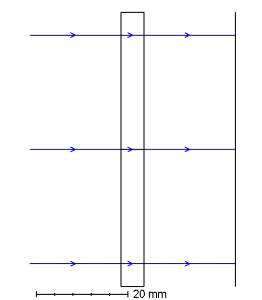
Practical Example: Flat Surface Sag Tolerance
Let’s consider a flat optical surface, commonly used in precision optical systems. If we wish to tolerance this surface with an RMS error of 1.0 micron, we use a Zernike Standard Sag surface and apply RMS tolerances accordingly.
In the TEZI tab:
- Maximum value: +1.0 micron
- Minimum value: -1.0 micron
This bidirectional range allows the simulation to generate positive or negative deviations, mimicking realistic manufacturing outcomes.
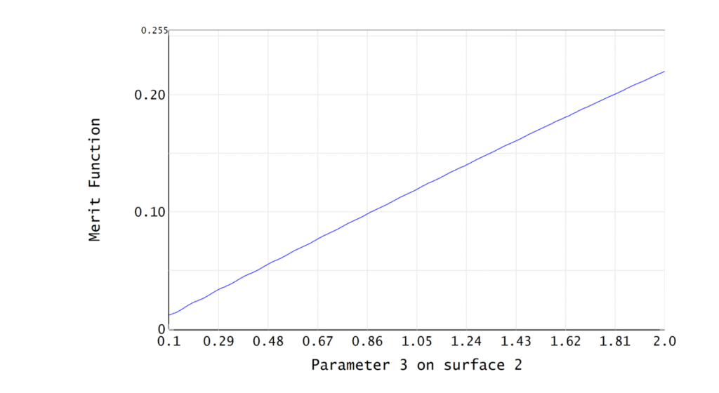
Zernike Order and Frequency: Selecting the Right Terms
The order of the Zernike polynomial terms directly impacts the simulated surface features:
| Zernike Term Range | Effect on Surface |
|---|---|
| Lower-order terms | Smooth, low-frequency distortions |
| Higher-order terms | Fine, high-frequency ripples |
For example:
- Terms 4 to 11 simulate broader undulations.
- Terms 12 to 28 introduce more localized, higher-frequency features.
At POC, we typically use up to term 28 to represent the manufacturing surface profile with sufficient accuracy for tolerance analysis.
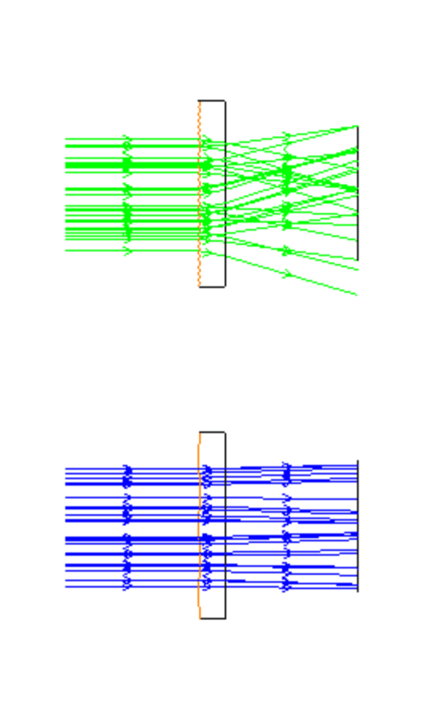
Surface Sag Simulation with Monte Carlo Analysis
We use Monte Carlo (MC) simulations to evaluate surface sag impacts across batches. By varying Zernike terms in each simulation run, we analyze how different spatial frequencies of sag influence system performance.
Observation: As we tighten surface flatness requirements (e.g., from 0.2 wavelength to 0.05 wavelength), the RMS error decreases, but the frequency of surface sag irregularities increases. This is a critical trade-off in balancing form error control and manufacturing complexity.